Map

 

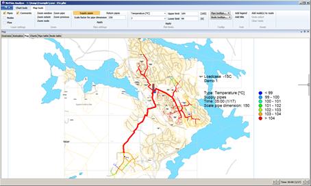
A map of the pipe network is created in the Map tab from the geometry description in the results file. A map background in DWG/DXF format can be loaded as a supplement to this screen.  Selected calculation results and input data are displayed as “tooltips” when the cursor is moved next to the object. Nodes are displayed as solid circles (green). Production plants are displayed in red. Nodes with consumption are displayed in magenta. Pipes are displayed with or without colours depending on whether or not the results plotting has been highlighted.

The Map tools panel is opened when you select the Map tab.

Layer settings

Here, you can select whether pipes, nodes, flows and comments are to be displayed or hidden.

Zoom

This commands can also be found in the right-click menu. Zoom pipe and zoom node highlight and centre the map over the pipe and node highlighted in Pipe table and node table respectively.

Pipe settings

Select whether the map is to display results for supply pipes or return pipes. Enter a value for scaling the pipe dimension (Scale factor for pipe dimension). A scale factor of 1 displays the pipe without scaling. 100 shows the pipe scaled with a 100 x dimension. Scaling allows you to see clearly which pipes have large and small dimensions. Apply your choice by pressing Apply.

Plot limit

Select the value to be plotted in the map. You can choose from flow (kg/s), velocity (m/s), temperature (°C), pressure (kPa), pressure difference (kPa), pressure level (kPa) and pressure gradient (Pa/m). Select the Don't show option if you do not want to display any results, just the pipe network. Select the number of colours (interval) to be used to display the results. Enter an upper limit and lower limit for the interval. The maximum and minimum values that appear in the results file are displayed in brackets adjacent to the fields. For example, if you specify 3 intervals and set the upper limit to 100 and the lower limit to 50, all values up to 50 will be displayed in one colour, all values from 50 to 100 will be displayed in the next colour, and all values above 100 will be displayed with the third colour. Apply your settings by pressing Apply.

 

Tooltip

When you move the cursor over a pipe or node in the map, calculation data can be displayed in a dialog box adjacent to the node/pipe. For pipes and nodes, select which data you want to view in the dialog box. For nodes, you can display name, level (m), pressure in supply and return pipe (kPa), temperature in supply and return pipe (°C), temperature difference (°C), flow from supply pipe to return pipe in the node (kg/s), bypass flow in the node (kg/s) and power (kW). For pipes, you can display name, diameter, pressure gradient in supply and return pipe (Pa/m), velocity in supply and return pipe (m/s), flow in supply and return pipe (kg/s) and heat loss value in supply and return pipe (W/m°C). 

 

Text

Select Add legend and point to the place in the map where you want to position your legend. If you want to move the legend, tag the command again and point to the new location. Select Add title if you want to display the headers from the model. You enter the headers in the calculation form in NetSim. (See also Legend window).

 

Route

This function is used to point out a route through the network along which you can display pressure, temperature and pressure gradient in a diagram. You have to enter the node at which the route is to start and where it should end. The routine itself finds the route through the network between the nodes which you indicated. The routine selects in a branch to follow the pipe with the biggest diameter. You can control the route which the routine selects by pointing to nodes which the route has to pass through before you point to the end node. The route selected by the routine is indicated in the map as you point. Remember, you can allow a route to pass to an end point and return from there by continuing to point to nodes. When you have started pointing to nodes with Add node(s) to route, the routine continues to select nodes as long as you continue to point to them. Finish pointing to nodes by pressing Esc. You can delete all nodes in the route by pressing clear route. If you have defined a route, you can add to this route by selecting Add node(s) to route or delete nodes by selecting Undo select.

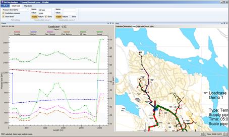
The Route function can also be found in the map's right-click menu.

 

Select object

The select object function, which can be found in the map's right-click menu, allows you to point to a pipe or node, and if you switch to the tab Pipe table or Node Table, the data for the selected object is highlighted in the table.

 

Clear selections

The clear selections function in the map's right-click menu deletes the highlights in the map which you saw when you opted to display highlighted pipes or nodes in the map in the Pipe table or Node Table tab.

 

Create animation

This function creates a slideshow from a time series calculation. See the section on time series calculations.

 

Background maps..

You can use this function to add background maps to your calculation. This function opens a dialog box where you select the map to be displayed. The format can be DWG, DXF or DGN. The dialog box remains open so that you can select more maps or delete maps which you have added as backgrounds.

 

Legend window:

In the right-click menu, you can enable a floating window which shows the interval limits in the map. 

.