Optimal weighting of weather
forecasts
Click on  above
“Selections” and click again on at
the bottom left of the dialog box displayed. Select “Automatic”. This changes
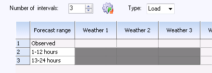
the behaviour for the grid at the top. You can select the cells instead of
typing numbers in the cells. If a cell is selected, this means for the current
forecast horizon that the corresponding selected forecast must be included as an
explanatory variable in the regression. Two regressions will be calculated in
the example below; one for the interval 13-24 hours, and one for 25-36 hours
ahead. Both of these will include forecasts from the suppliers “Weather 1”,
“Weather 2” and “Weather 3” as explanatory variables. The program will
automatically enter weights for the forecast horizons not selected so that the
calculated weights for row 3 will be copied to rows 1 and 2. Likewise, if this
weighting is to be evaluated for more than 36 hours ahead, the “25-36” hour
weighting will be used. These calculations are time-consuming, and there may be
a need to limit the number of regressions to the forecast horizons for which you
are most in need of minimising balance errors.
above
“Selections” and click again on at
the bottom left of the dialog box displayed. Select “Automatic”. This changes
the behaviour for the grid at the top. You can select the cells instead of
typing numbers in the cells. If a cell is selected, this means for the current
forecast horizon that the corresponding selected forecast must be included as an
explanatory variable in the regression. Two regressions will be calculated in
the example below; one for the interval 13-24 hours, and one for 25-36 hours
ahead. Both of these will include forecasts from the suppliers “Weather 1”,
“Weather 2” and “Weather 3” as explanatory variables. The program will
automatically enter weights for the forecast horizons not selected so that the
calculated weights for row 3 will be copied to rows 1 and 2. Likewise, if this
weighting is to be evaluated for more than 36 hours ahead, the “25-36” hour
weighting will be used. These calculations are time-consuming, and there may be
a need to limit the number of regressions to the forecast horizons for which you
are most in need of minimising balance errors.
When you change the weighting from “Manual” to “Automatic”,
a range of options will be displayed in the dialog box. The step-wise regression
allows you to remove weather forecasts which do not make a sufficient
contribution to the explanation of the outcome. As a first step, the step-wise
regression algorithm used identifies the forecast which alone can explain as
much as possible of the variation of the historical outcome. After this forecast
is included, a search is carried out for the remaining forecasts which one
alone can describe most of the remaining variation.
In a third step, a search is carried out for the remaining
forecast which best explains what now remains of the outcome to be explained,
and so on.
After a number of steps, the inclusion of a new forecast
will only marginally improve the results, and this improvement can be purely
randomly induced by conditions during the evaluation period.
The stopping criteria for the step-wise parameter selection
procedure are 2 significance test (F-tests). There is a certain degree of
uncertainty with every statistical test, and we have decide what risk we are
prepared to accept in the significance test.
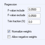
In the “Regression” box, you can enter:
•
F-value include: Enter the risk you are prepared to
take of including a new variable totally uncorrelated with the historical
outcome. If you want it not to accept errors more frequently than in 5% of
cases, enter 0.05 under the header “F-value include”.
•
F-value exclude: The step-wise algorithm also has the option
to throw out a variable which was important in an earlier step but which is no
longer important when another one or more variables have been added. The risk
you want to take of not throwing out a previously totally uncorrelated variable
with the historical outcome is specified under the header:
“F-value exclude”. A value higher than “F-value include”
will give a conservative model which generally does not throw out variables
which have already been included.
•
Trim fraction: The exact proportion of extreme values that are to
be excluded from the regression. The entire interval between the forecast
minimum value of the evaluation period and its maximum value is divided up into
a number of sub-intervals. For each sub-interval the highest and lowest measured
values are removed from the regression. A high value gives regression results
towards a minimization of the mean absolute error (MAE), in contrast to an
ordinary regression (value 0) that minimises RMSE.
•
Normalize weights: The result of a regression normally gives a
total of the weights which differs from 100% and a constant non-zero term. This
may be justified as forecasts for a specific forecast horizon may systematically
deviate from the observed weather on which the forecast models are trained. If,
instead, you want the result to reflect a “trust” you have for the various
weather forecasts, you can check this check box. The total of the weights can
then be scaled up to 100% and the constant is omitted.
•
Allow negative weights: The linear regression can also result in
negative weights. Uncheck this if these are not to be permitted.
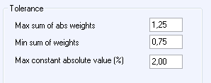
The “Tolerance” box contains options for defining settings
for warning messages from the regression process. Normally, the results from
regression should give positive weights (possibly also a slight negative) which
are close to 1 when totalled. The constant should also be small in relation to
the mean load. Deviations from this may indicate problems somewhere in the
forecast processes.
•
Max sum of abs weights: If you allow negative weights, the
absolute sum of individual weights may be significantly higher than 100% even if
the total of weights is close to 100%. For example, a regression may set 200%
weight on forecast 1 and -100% on forecast 2. Set the highest accepted total of
the absolute sums of the weights.
•
Min sum of weights: The program issues a warning if the sum of
weights falls below this value.
•
Max constant absolute value: The program issues a warning if the
absolute value of the constant estimated during regression exceeds the specified
percentage (percentage of the mean load during the evaluation period).
When we are satisfied with our settings, these are saved as
a “Selection” which then can evaluate. During evaluation, you will first
calculate the optimal weights for all forecast series for all series you
selected. In step two, these will then be evaluated for the forecast horizons
entered in an “extract”.