 to the left of it. To reset the
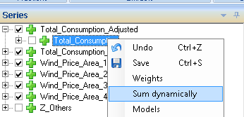
aggregation relation, right-click on the subseries you want to dynamically
aggregate and select “Sum dynamically”.
to the left of it. To reset the
aggregation relation, right-click on the subseries you want to dynamically
aggregate and select “Sum dynamically”.Resetting to dynamic fractions must be performed from a
subseries that is aggregated without fractions, i.e. has to the left of it. To reset the
aggregation relation, right-click on the subseries you want to dynamically
aggregate and select “Sum dynamically”.
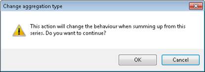
Click on OK in the warning window that pops up.
The plus symbol is then replaced with  and a diskette symbol to the right of the
series indicates that the change has not yet been permanently saved. Save the
change by right-clicking again on the same series and select “Save”.
and a diskette symbol to the right of the
series indicates that the change has not yet been permanently saved. Save the
change by right-clicking again on the same series and select “Save”.
Just as in the case of ordinary fractions, the circles
displayed to the left of the series indicate how large a fraction of the series
is aggregated to the next level. A fully-shaded blue circle corresponds to 100%, so that in practice
the series is still aggregated in exactly the same way as with the previous . To change settings for the aggregation,
right-click on the aggregated series for the series we recently reset to dynamic
aggregation.
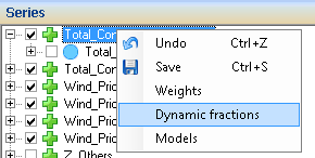
Select “Dynamic fractions”. The following dialog box will be displayed.
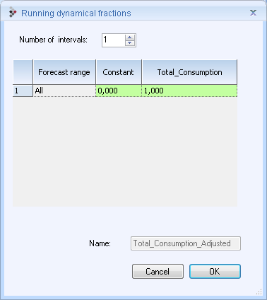
At the very top of the dialog box (“Number of intervals:”), select the number of 12-hour intervals into which you want to split the forecast period. Each interval corresponds to a row in the “grid”, and in the “Forecast range” column, enter the hours, calculated from forecast start, for which the values in the row will apply. You can enter values either as a constant or as a factor that is to be multiplied by all the forecast values of the subseries. If the aggregated series has several subseries dynamically connected to it, a column for each series will be displayed. The unit of the constant is controlled by the system setting and also depends on the time resolution. If the set magnitude is energy, the time resolution is 30 minutes and he constant is 1, this means that 1 MWh is to be added to the aggregated series for each half hour. If the time resolution is later changed to 15 minutes and the same dialog box is displayed, the value of the constant will be halved, as only 0.5 MWh is to be added each separate quarter of an hour.
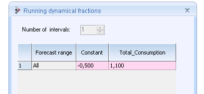
In the dialog box above, the value of the constant is -0.5
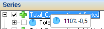
and the factor 1.1. has been entered. Once you have clicked on “OK”,  is instead displayed to the left of the series
“Total_Consumption” (values above 100% are shown as darker blue segments of a
lighter shaded circle). When you hover the cursor above the circle, the factor
and constant are also shown numerically as below.
is instead displayed to the left of the series
“Total_Consumption” (values above 100% are shown as darker blue segments of a
lighter shaded circle). When you hover the cursor above the circle, the factor
and constant are also shown numerically as below.
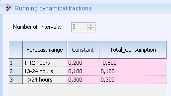
You can also let the dynamic fractions vary over time, in which case the hours are always calculated from the start of the forecast. Below, hours 1 to 12 will be aggregated according to the constant 0.2 and the negative factor -0.5, then, between hours 13 and 24, according to the constant 0.1 and the factor 0.1, and, after 24 hours, the constant 0.3 and the factor 0.3 will be used.
Exactly which segment icon is shown is determined by the
first factor, and since the first factor here is negative, a red segment  will be displayed in the series tree
instead of a blue one.
will be displayed in the series tree
instead of a blue one.