Assume that you have for a time evaluated the forecasts for an aggregated series and noticed some degree of systematic deviation from the measured values. Normally you should in that case be able to identify the reason for this in the forecasts for one or more of the subseries of this series. Generally, you can then change the model settings for these so as to eliminate the deviations. However, if it tends to be the case that the deviations occur through the aggregation rather than that the individual errors from the subseries (which may be regarded as unsystematic) are being added up to give systematic errors, such errors can be reduced by the use of dynamic fractions. An example might be the sum of wind forecasts, where uncertainty in each individual wind forecast results in the model for the production forecast being – for good reason – “cautious”, i.e. varying less than the measured production. But the sum of these “cautious” forecasts may be unnecessarily cautious. Sudden upturns and downturns are difficult to plot in at the correct time for the individual plants, and smoothing effects generally make it easier to forecast upturns and downturns for the total production within an area. Dynamic fractions make it possible to adjust forecasts in retrospect after or during the aggregation process. In the previous section we showed how you can manually correct an aggregated forecast (“Total_Consumption”) at the time of aggregation with the result of the correction saved for the aggregated series at the very top of the tree structure (“Total_consumption_adjusted”).
Here instead we intend to use linear regression during an ordinary evaluation to calculate the optimum linear correction for the desired time interval.
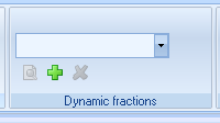
We start by going to the “Follow Up” tab and clicking on
 in “Dynamic fractions”. A dialog box
like the one below appears:
in “Dynamic fractions”. A dialog box
like the one below appears:
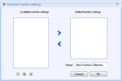
This dialog box is used to select which created settings we
will use for a given evaluation. Click on bottom left to create the appropriate
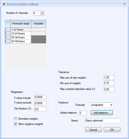
setting template. At the top of the dialog box that then appears you can select
the forecast intervals for which you want an optimum correction calculated.
Assume that you produce a forecast each day that starts at hour 1 of the day in
question. The part of the forecast used for power trading will in that case be
hours 25-48 for the electricity spot market.
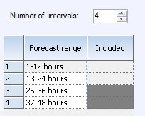
Select 4 intervals and click in the boxes for “Included” to the right of “25-36 hours” and “37-48 hours”. We have now selected the option of calculating an optimum correction for the first 12 hours of electricity spot trading and a different optimum correction for the last 12 hours. All hours for boxes left empty (1-24 hours) will be given the same correction as 25-36, and for hours above 48, the 37-48 hours correction applies.
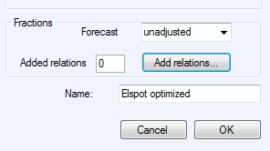
You can read about other settings that apply to the linear regression in the section entitled “Optimum weighting of weather forecasts”.
The remaining settings that are specific to these in particular are:

1. Linear correction of an aggregated forecast
2. Weight together alternative forecasts for a forecast series
3. Evaluate different weather forecasts
4. Change weighting for live forecasts