First, we select the series that we want to evaluate in the tree structure.  The selected series are the only ones for which results will be displayed. In other words, results for subseries for a preselected series will not be displayed automatically in contrast to how forecasts are displayed.

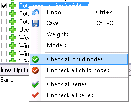
 Often, we want to evaluate series on a lower aggregated level than the exported series. To check or uncheck all sub series for a node in the tree structure, just right-click on the node and select ‘Check all child nodes’. Undo the selection by ‘Uncheck all child nodes’.

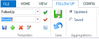
We can create a template, by using the ‘Templates’ control and also separate the templates used for follow up with templates used for other purposes by specifying the template type to ‘FollowUp’ as in the picture below.

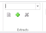
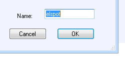
For the program to be able to find the right forecast files and extract the right data from these when a period is to be evaluated, we need settings which define how the program should search for data to extract. These settings are found in the ‘Extracts’ control.  Each evaluation can use a number of these extract settings simultaneously. We will begin by creating a collection of extract settings which we will call “elspot”. Start by clicking on  above ‘Extracts’.

In the dialog box displayed, we click on  at the bottom left. The following dialog box is then displayed, where we can create an extract setting.

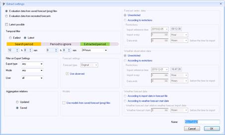
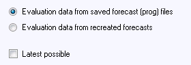
To the top left, we have the option of either evaluate saved or recreated forecasts. Recreated forecasts are described in the section ‘Evaluation of recreated forecasts’. 

When evaluating a period, it will be divided into a number of sub-periods.In the ’Temporal filter’, we can filter out prog-files based on when they were saved relative to the evaluated sub periods.

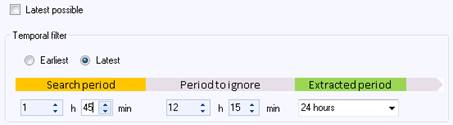
 If we want each day to be evaluated with a forecast created between 10:00 and 11:45 the day before, we can first set ‘Extracted period’ to 24 hours, i.e. each day is evaluated at a time. ‘Period to ignore’ is set to 12 hours and 15 minutes and ‘Search period’ is set to 1 hour and 45 minutes. When the program will evaluate a certain day, e.g. 2016-03-05, it will search for a forecast saved between 10:00 and 11:45 the day before, i.e. 2016-03-04. All values for the 5^th  of March will be extracted from the first  file found that matches the additional search criteria. Values for all of 02-03-2012 will be evaluated from this forecast. If no such file is found or if the file lack some forecast values for the desired day, this will lead to a gap of missing values in the evaluated data. If ‘Latest possible’ is checked, the ‘Temporal filter’ settings will be greyed.

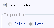
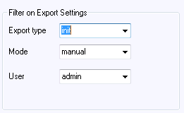
In that case, the program will search for all files during the evaluation period, extract all data from all files and constructs a time series by going forward in time, overwriting data from older files with data from newer files.  Further down, we can filter out forecasts which do not interest us by selecting under “Export type” a special type of export which does interest us and selecting under “Mode” if you only want automatic forecasts or only forecasts exported manually to be evaluated. Evaluations can also be made for forecasts made by specific users. Select “any” here if the program shouldn’t take these parameters into account.

Set ‘Aggregation relations’ to ‘Saved’ (more about this in the sections   ‘Evaluate preliminary fractions with final ones’  and  ‘Evaluation of aggregated series ’). When we are happy with our settings, type “elspot” in the name field and click on OK.

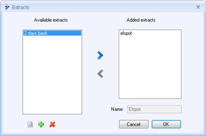
At this point, “elspot” is displayed as an available extract in the earlier dialog box below. Clicking on allows you to select whether the newly created extract is to be included in the current extract collection.  Clicking on  and changes, creates new or deletes extracts, and the andarrows are used to add extracts to and delete extracts from the current extract collection. Our collection will only include the “elspot” extract, so we type “elspot” in the name box for the selection and click on OK.

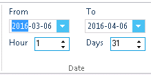
We then select an evaluation period with the start date at the top and the number of days in the “Days” box or specify the end date instead. Also we should set ‘Hour’ to something else than ‘1’ if for example our data is in EET (GMT+2h) but we want to evaluate trading on the NordPool market which is in CET (GMT+1h).

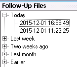
   We can use the list of saved forecasts to check that there are forecasts saved for the period we selects.

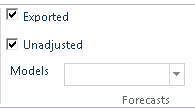
There are two check boxes in the “Forecasts” control to the right of the “Date” control.  If the “Exported” check box is checked, the exported forecast will be evaluated, i.e. including the manual adjustments of the forecast made by the exported forecast. If the “Unadjusted” check box is checked, the unadjusted forecast will also be evaluated. We will check both.

We can skip the “Selection” field to the right of “Forecasts” for the moment, and click directly on    to start the evaluation. While evaluation is in progress, a display at the bottom left indicates how far it has progressed.

 To cancel the evaluation, click on .

When the evaluation is complete, three curves will be displayed in the top diagram. The black one is the actual result which can be compared with the exported data and the unadjusted forecast. The illustration below shows an example of how an enhancing adjustment has been carried out by the forecast on the right in the diagram.

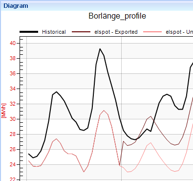
The bottom diagram shows corresponding weather parameters in which the forecast values can be compared with observed weather. If you want to delete certain parameters, you can go back to the “View” tab and uncheck the relevant check boxes. When you then click back to “Follow-Up”, only the parameters that you left checked will be displayed. A spreadsheet containing the corresponding values in numerical format is shown on the right. The “Statistics” window appears at the bottom right, showing a few forecast quality measures.

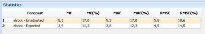
These are:

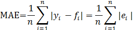
•      the ME (Mean Error) given by

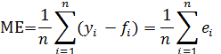
where e_i=y_i-f_iis the ith error. A positive mean error indicates that the forecasts are too low on average.

•      MAE (Mean Absolute Error), quite simply the average of the absolute total of the errors. This dimension has a natural link to actual balance costs.

•      RMSE (Root of Mean Squared Errors),

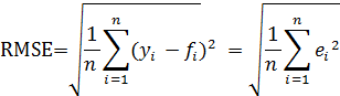
which is found by taking the square root of the mean value of the squared errors. By definition, this dimension will be greater than MAE. A high RMSE compared with MAE indicates uneven forecast quality.

•      MAX AE (Max Absolute error)

The maximum value of the absolute errors

•      COUNTS

Number of observations with non-missing values

All these measures are given both as absolute measures (energy or output) and as a percentage of the mean load during the evaluated period.